
There are still many useful tips and tricks that are inevitably overlooked. Here are 20 useful Excel spreadsheet secrets you may not know and also Numpad codes
1. One Click to Select All
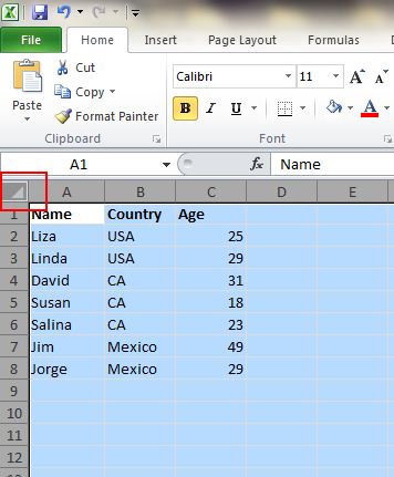
You might know how to select all by using the Ctrl + A shortcut, but few know that with only one click of the corner button, as shown in the screenshot below, all data will be selected in seconds.
2. Open Excel Files in Bulk
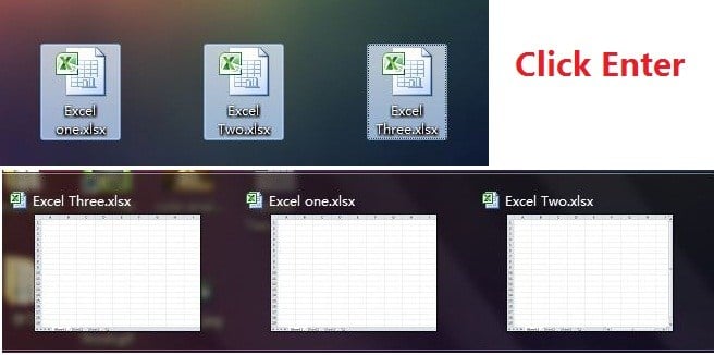
Rather than open files one by one when you have multiple files you need to handle, there is a handy way to open them all with one click. Select the files you would like to open then press the Enter key on the keyboard, all files will open simultaneously.
3. Shift Between Different Excel Files
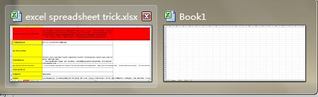
When you have different spreadsheets open, it’s really annoying shifting between different files because sometimes working on the wrong sheet can ruin the whole project. Using Ctrl + Tab you can shift between different files freely. This function is also applicable to other files like different Windows tabs in Firefox when opened using Windows 7.
4. Create a New Shortcut Menu
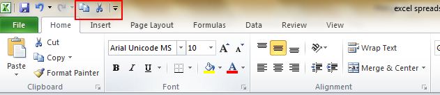
Generally there are three shortcuts in the top menu, which are Save, Undo Typing and Repeat Typing. However, if you want to use more shortcuts, like Copy and Cut, you can set them up as follows:
File->Options->Quick Access Toolbar, add Cut and Copy from the left column to the right, save it. You will see two more shortcuts added in the top menu.
5. Add a Diagonal Line to a Cell
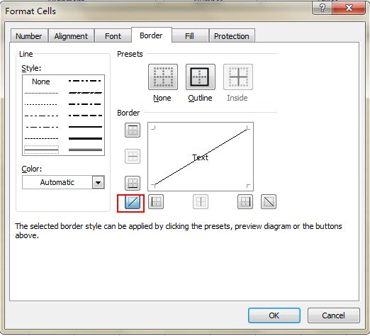
When creating a classmate address list, for example, you may need a diagonal link in the first cell to separate different attributes of rows and columns. How to make it? Everyone knows that Home->Font-> Borders can change different borders for a cell, and even add different colors. However, if you click More Borders, you will get more surprises, like a diagonal line. Click it and save—you can now make it immediately.
6. Add More Than One New Row or Column
You may know the way to add one new row or column, but it really wastes a lot of time if you need to insert more than one of these by repeating this action X number of times. The best way is to drag and select X rows or columns (X is two or more) if you want to add X rows or columns above or left. Right click the highlighted rows or columns and choose Insert from the drop down menu. New rows will be inserted above the row or to the left of the column you first selected.
7. Speedily Move and Copy Data in Cells
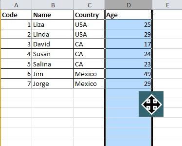
If you want to move one column of data in a spreadsheet, the fast way is to choose it and move the pointer to the border, after it turns to a crossed arrow icon, drag to move the column freely. What if you want to copy the data? You can press the Ctrl button before you drag to move; the new column will copy all the selected data.
8. Speedily Delete Blank Cells
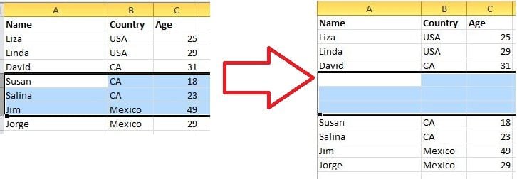
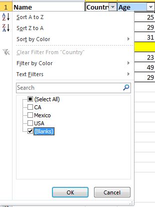
Some default data will be blank, for various reasons. If you need to delete these to maintain accuracy, especially when calculating the average value, the speedy way is to filter out all blank cells and delete them with one click. Choose the column you want to filter, go to Data->Filter, after the downward button shows, undo Select All and then pick up the last option, Blanks. All blank cells will show immediately. Go back to Home and click Delete directly, all of them will be removed.
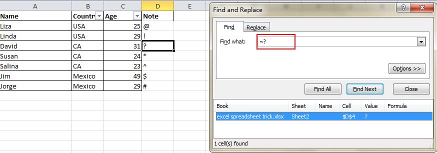
9. Vague Search with Wild Card
You may know how to activate the speedy search by using the shortcut Ctrl + F, but there are two main wild cards—Question Mark and Asterisk—used in Excel spreadsheets to activate a vague search. This is used when you are not sure about the target result. Question Mark stands for one character and Asterisk represents one or more characters. What if you need to search Question Mark and Asterisk as a target result? Don’t forget add a Wave Line in front.
10. Generate a Unique Value in a Column
You are aware of the key function of Filter, but few people use the Advanced Filter, which will be repeatedly applied when you need to filter a unique value from data in a column. Click to choose the column and go to Data->Advanced. A pop-up window will show up. As the screenshot shows, click Copy to another location, which should be in accord with the second red rectangular area. Then specify the target location by typing the value or clicking the area-choosing button. In this example, the unique age can be generated from Column C and show in Column E. Don’t forget to choose Unique records only, then click OK. The unique value showing in column E can be the contrast of the original data in C, that’s the reason why it is recommended to copy to another location.

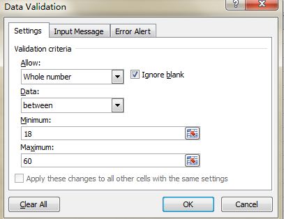
11. Input Restriction with Data Validation Function
In order to retain the validity of data, sometimes you need to restrict the input value and offer some tips for further steps. For example, age in this sheet should be whole numbers and all people participating in this survey should be between 18 and 60 years old. To ensure that data outside of this age range isn’t entered, go to Data->Data Validation->Setting, input the conditions and shift to Input Message to give prompts like, “Please input your age with whole number, which should range from 18 to 60.” Users will get this prompt when hanging the pointer in this area and get a warning message if the inputted information is unqualified.
12. Fast Navigation with Ctrl + Arrow Button
When you click Ctrl + any arrow button on the keyboard, you can jump to the edge of the sheet in different directions. If you want to jump to the bottom line of the data, just try to click Ctrl + downward button.

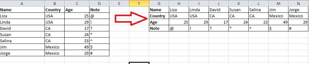
13. Transpose Data from a Row to a Column
You would use this feature if you want to transpose data to get a better display; however, retyping all data would be the last thing you would need to do if you know how to use the Transpose function in Paste. Here’s how: copy the area you want to transpose, move the pointer to another blank location. Go to Home->Paste->Transpose, please note that this function won’t activate until you copy the data first.
14. Hide Data Thoroughly
Almost all users know how to hide data by right clicking to select the Hide function, but this can be easily noticed if there is only a little bit of data. The best and easiest way to hide data thoroughly is to use the Format Cells function. Choose the area and go to Home->Font->Open Format Cells->Number Tab->Custom->Type ;;; -> Click OK, then all the values in the area will be invisible, and can only be found in the preview area next to the Function button.
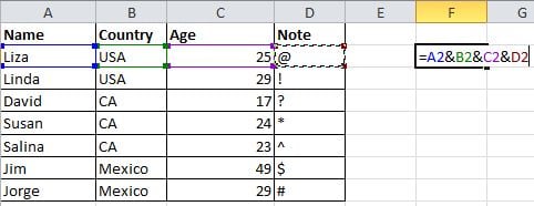
15. Compose Text with &
Complicated formulation is unnecessary, as long as you know how to use &. You can compose any text freely with this symbol. Below I have four columns with different texts, but what if I want to compose them to one value in one cell? First, locate the cell that is to show the composed result, use the formulation with & as shown in the screenshot below. Click Enter: all texts in A2, B2, C2 and D2 will be composed together to become LizaUSA25@ in F2.
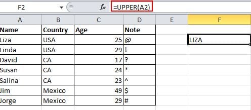
16. Transforming the Case of Text
With all the tricks shared here, I’ve tried my best to avoid complicated formulation. But there are still some simple and easy to use formulations to show you, like UPPER, LOWER and PROPER, which can transform texts for different purposes. UPPER will capitalize all characters, LOWER can change text to all lower case and PROPER will only capitalize the first character of a word.
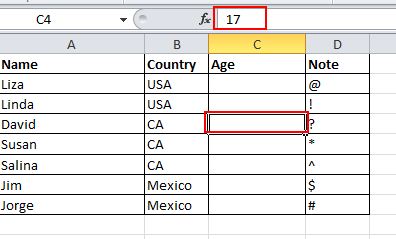
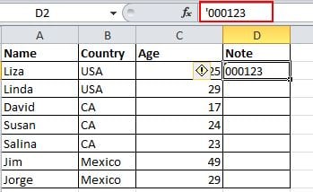
17. Input Values Starting with 0
When an input value starts with zero, Excel will delete the zero by default. Rather than reset the Format Cells, this problem can be easily solved by adding a single quote mark ahead of the first zero, as shown.
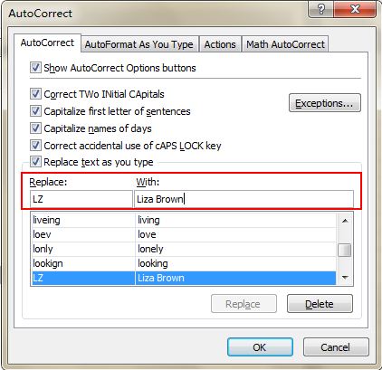
18. Speed up Inputting Complicated Terms with AutoCorrect
If you need to repeat the same value and it is complicated to input, the best way is to use the AutoCorrect function, which will replace your text with the correct text. Take my name, Liza Brown, for example, which can be replaced by LZ. Therefore, every time I input LZ, it can autocorrect to Liza Brown. Go to File->Options->Proofing->AutoCorrect Options and input Replace text with correct text in the red rectangular area, as below.
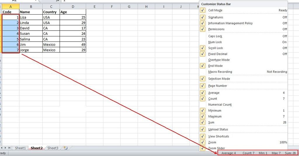
19. One Click to Get More Status
Most users know how to check the data status in the bottom of an Excel sheet, like Average and Sum Value. However, do you know you can move the pointer to the bottom tab and right click to get more status, as shown below?
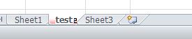
20. Rename a Sheet Using Double Click
There are multiple ways to rename sheets, and most users will right click to choose Rename, which actually wastes a lot of time. The best way is to just click twice, then you can rename it directly.
Want to level up your excel skills further? Don’t miss this article
21. Numpad Codes
Im I'm only covering the first 256 characters of both sets in my chart, in some cases you can go higher but it depends on the application you are typing in. For example, ALT+257 gives me ā in Wordpad, but in Notepad it loops back around the character set and gives me☺(257-256=1 which is ☺ in the OEM set) . If you want to know what key code will bring up a particular character in a certain Windows font run Windows Character Map (charmap.exe) and look in the bottom right corner to find out.
|
|
|
|
Comments
Post a Comment